Example 1: Basic Mann Model Fit

This example demonstrates fitting the Mann model eddy lifetime function to the Kaimal one-point spectra and cross-spectra.

For reference, the Mann eddy lifetime function is given by

\begin{align}\tau^{\mathrm{Mann}}(k)=\frac{(k L)^{-\frac{2}{3}}}{\sqrt{{ }_2 F_1\left(1 / 3,17 / 6 ; 4 / 3 ;-(k L)^{-2}\right)}}\,.\end{align}

This set of models it widely used for flat, homogeneous terrains.

drdmannturb can also be used directly to generate the corresponding 3D turbulence field, as demonstrated in Examples 8 and 9.

Import packages

First, we import the packages needed for this example.

import torch

from drdmannturb import EddyLifetimeType
from drdmannturb.parameters import (
    LossParameters,
    NNParameters,
    PhysicalParameters,
    ProblemParameters,
)
from drdmannturb.spectra_fitting import CalibrationProblem, OnePointSpectraDataGenerator

device = "cuda" if torch.cuda.is_available() else "cpu"

if torch.cuda.is_available():
    torch.set_default_tensor_type("torch.cuda.FloatTensor")

Set up physical parameters and domain. We perform the spectra fitting over the \(k_1 z\) space \([10^{{-1}}, 10^2]\) with 20 points.

zref = 40  # reference height
ustar = 1.773  # friction velocity

# Intitial parameter guesses for fitting the Mann model
L = 0.59 * zref  # length scale
Gamma = 3.9  # time scale
sigma = 3.2 * ustar**2.0 / zref ** (2.0 / 3.0)  # magnitude (σ = αϵ^{2/3})

print(f"Physical Parameters: {L,Gamma,sigma}")

k1 = torch.logspace(-1, 2, 20) / zref

Physical Parameters: (23.599999999999998, 3.9, 0.8600574364289042)

CalibrationProblem Construction

The following cell defines the CalibrationProblem using default values for the NNParameters and LossParameters dataclasses. Notice that EddyLifetimeType.MANN specifies the Mann model for the eddy lifetime function, \(\tau\), meaning no neural network is used in learning \(\tau\). Thus, we only learn the parameters \(L\), \(\Gamma\), and \(\sigma\).

pb = CalibrationProblem(
    nn_params=NNParameters(),
    prob_params=ProblemParameters(eddy_lifetime=EddyLifetimeType.MANN, nepochs=2),
    loss_params=LossParameters(),
    phys_params=PhysicalParameters(
        L=L, Gamma=Gamma, sigma=sigma, ustar=ustar, domain=k1
    ),
    device=device,
)

Data Generation

We now collect Data = (<data points>, <data values>) and specify the reference height (zref) to be used during calibration. Note that DataType.KAIMAL is used by default.

Data = OnePointSpectraDataGenerator(data_points=k1, zref=zref, ustar=ustar).Data

The model is now fit to the provided spectra given in Data.

Notee that the Mann eddy lifetime function relies on evaluating a hypergeometric function, which only has a CPU implementation through Scipy; cf. Example 7.

Having the necessary components, the model is “calibrated” (fit) to the provided spectra.

optimal_parameters = pb.calibrate(data=Data)

========================================
Initial loss: 0.036969418218857554
========================================

100%|██████████████████████████████████████████████████████████████████| 2/2 [00:07<00:00,  3.53s/it]

========================================
Spectra fitting concluded with final loss: 0.025248721189996617

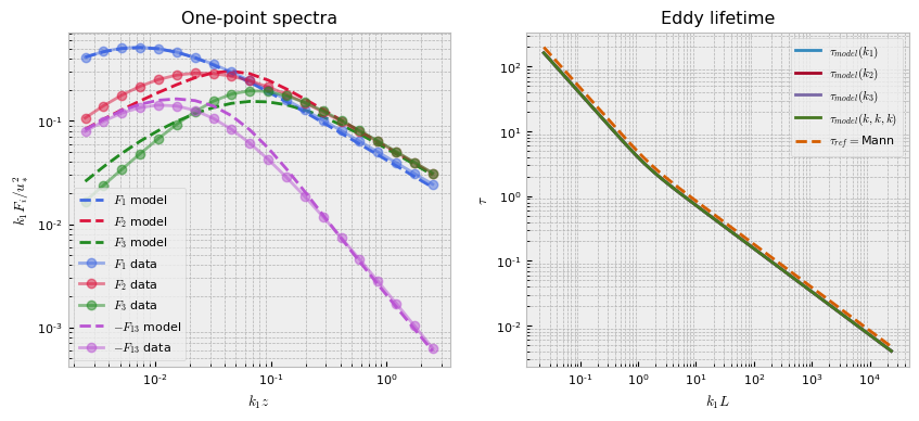
We conclude by printing the optimized parameters and generating a plot showing the fit to the Kaimal spectra.

pb.print_calibrated_params()
pb.plot()

========================================
Optimal calibrated L        :  27.2532 
Optimal calibrated Γ        :   3.6762 
Optimal calibrated αϵ^{2/3} :   0.7988 
========================================