Example 2: Synthetic Data Fit

In this example, we compare the DRD model to the Mann model, using the three IEC-recommended Mann model parameters: \(L/\text{zref}=0.59, Γ=3.9, αϵ^{2/3}=3.2 * (\text{zref}^{2/3} / \text{ustar}^2)\). In this example, the exponent \(\nu=-\frac{1}{3}\) is fixed so that \(\tau(\boldsymbol{k})\) matches the slope of \(\tau^{IEC}\) for in the energy-containing range, \(k \rightarrow 0\).

The following example is also discussed in the original DRD paper.

Import packages

First, we import the packages we need for this example. Additionally, we choose to use CUDA if it is available.

import torch
import torch.nn as nn

from drdmannturb import EddyLifetimeType
from drdmannturb.parameters import (
    LossParameters,
    NNParameters,
    PhysicalParameters,
    ProblemParameters,
)
from drdmannturb.spectra_fitting import CalibrationProblem, OnePointSpectraDataGenerator

device = "cuda" if torch.cuda.is_available() else "cpu"

if torch.cuda.is_available():
    torch.set_default_tensor_type("torch.cuda.FloatTensor")

Setting Physical Parameters

The following cell sets the necessary physical parameters

\(L\) is our characteristic length scale, \(\Gamma\) is our characteristic time scale, and \(\sigma = \alpha\epsilon^{2/3}\) is the spectrum amplitude.

zref = 90  # reference height
z0 = 0.02
zref = 90
uref = 11.4
ustar = 0.556  # friction velocity

# Scales associated with Kaimal spectrum
L = 0.593 * zref  # length scale
Gamma = 3.89  # time scale
sigma = 3.2 * ustar**2.0 / zref ** (2.0 / 3.0)  # magnitude (σ = αϵ^{2/3})

print(f"Physical Parameters: {L,Gamma,sigma}")

k1 = torch.logspace(-1, 2, 20) / zref

Physical Parameters: (53.37, 3.89, 0.04925737023046032)

CalibrationProblem construction

We’ll use a simple neural network consisting of two layers with \(10\) neurons each, connected by a ReLU activation function. The parameters determining the network architecture can conveniently be set through the NNParameters dataclass.

Using the ProblemParameters dataclass, we indicate the eddy lifetime function \(\tau\) substitution, that we do not intend to learn the exponent \(\nu\), and that we would like to train for 10 epochs, or until the tolerance tol loss (0.001 by default), whichever is reached first.

Having set our physical parameters above, we need only pass these to the PhysicalParameters dataclass just as is done below.

Lastly, using the LossParameters dataclass, we introduce a second-order derivative penalty term with weight \(\alpha_2 = 1\) and a network parameter regularization term with weight \(\beta=10^{-5}\) to our MSE loss function.

pb = CalibrationProblem(
    nn_params=NNParameters(
        nlayers=2,
        # Specifying the hidden layer sizes is done by passing a list of integers, as seen here.
        hidden_layer_sizes=[10, 10],
        # Specifying the activations is done similarly.
        activations=[nn.ReLU(), nn.ReLU()],
    ),
    prob_params=ProblemParameters(
        nepochs=10, learn_nu=False, eddy_lifetime=EddyLifetimeType.TAUNET
    ),
    # Note that we have not activated the first order term, but this can be done by passing a value for ``alpha_pen1``
    loss_params=LossParameters(alpha_pen2=1.0, beta_reg=1.0e-5),
    phys_params=PhysicalParameters(
        L=L, Gamma=Gamma, sigma=sigma, ustar=ustar, domain=k1
    ),
    logging_directory="runs/synthetic_fit",
    device=device,
)

Data Generation

We now collect Data = (<data points>, <data values>) and specify the reference height (zref) to be used during calibration. Note that DataType.KAIMAL is used by default.

Data = OnePointSpectraDataGenerator(data_points=k1, zref=zref, ustar=ustar).Data

Calibration

Now, we fit our model. CalibrationProblem.calibrate takes the tuple Data which we just constructed and performs a typical training loop.

optimal_parameters = pb.calibrate(data=Data)

pb.print_calibrated_params()

========================================
Initial loss: 0.04606855911763526
========================================

100%|████████████████████████████████████████████████████████████████| 10/10 [00:21<00:00,  2.19s/it]

========================================
Spectra fitting concluded with final loss: 0.008501029301051776
========================================
Optimal calibrated L        :  54.5565 
Optimal calibrated Γ        :   1.4951 
Optimal calibrated αϵ^{2/3} :   0.0460 
========================================

Plotting

DRDMannTurb offers built-in plotting utilities and Tensorboard integration which make visualizing results and various aspects of training performance very simple.

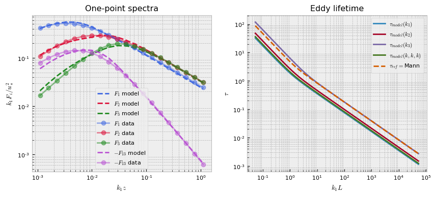
The following will plot the fit.

pb.plot()

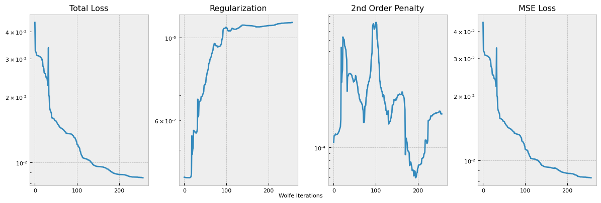
This plots out the loss function terms as specified, each multiplied by the respective coefficient hyperparameter. The training logs can be accessed from the logging directory with Tensorboard utilities, but we also provide a simple internal utility for a single training log plot.

pb.plot_losses(run_number=0)

Save Model with Problem Metadata

Here, we’ll make use of the model saving utilities, which make saving the DRDMannTurb fit very straightforward. The following line automatically pickles and writes out a trained model along with the various parameter dataclasses in ../results.

pb.save_model("./outputs/")

Loading Model and Problem Metadata

Lastly, we load our model back in.

import pickle

path_to_parameters = "./outputs/EddyLifetimeType.TAUNET_DataType.KAIMAL.pkl"

with open(path_to_parameters, "rb") as file:
    (
        nn_params,
        prob_params,
        loss_params,
        phys_params,
        model_params,
    ) = pickle.load(file)

Recovering Old Model Configuration and Old Parameters

We can also load the old model configuration from file and create a new CalibrationProblem object from the stored network parameters and metadata.

pb_new = CalibrationProblem(
    nn_params=nn_params,
    prob_params=prob_params,
    loss_params=loss_params,
    phys_params=phys_params,
    device=device,
)

pb_new.parameters = model_params

import numpy as np

assert np.ma.allequal(pb.parameters, pb_new.parameters)