Example 6: Interpolating Spectra Data and Fitting

In this example, we’re using real-world data, but importantly the data points are not over the same spatial coordinates. Since that congruency is required, we need to interpolate the data values and obtain them over a common set of points. Furthermore, we filter the noisy data to obtain smoother curves for the DRD model to fit. DRDMannTurb has built-in utilities for handling this.

This process involves new sources of error: interpolation error and filtering error, in addition to the sources from data collection and DRD model training.

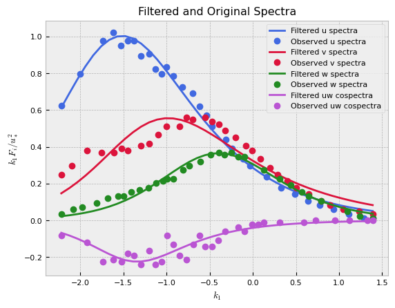
The filtering is based on differential evolution to perform a non-linear fit onto functions of the following form:

\begin{align}\frac{k_1 F_{11}\left(k_1 z\right)}{u_*^2}=J_1(f):=\frac{a_1 f}{(1+b_1 f)^{c_1}}\end{align}

\begin{align}\frac{k_1 F_{22}\left(k_1 z\right)}{u_*^2}=J_2(f):=\frac{a_2 f}{(1+b_2 f)^{c_2}}\end{align}

\begin{align}\frac{k_1 F_{33}\left(k_1 z\right)}{u_*^2}=J_3(f):=\frac{a_3 f}{1+ b_3 f^{ c_3}}\end{align}

\begin{align}-\frac{k_1 F_{13}\left(k_1 z\right)}{u_*^2}=J_4(f):=\frac{a_4 f}{(1+ b_4 f)^{c_4}}\end{align}

with \(F_{12}=F_{23}=0\). Here, \(f = (2\pi)^{-1} k_1 z\). In the above, the \(a_i, b_i, c_i\) are free parameters which are optimized by differential evolution. The result is a spectra model that is similar in form to the Kaimal spectra and which filters/smooths the spectra data from the real world and eases fitting by DRD models. This option is highly suggested in cases where spectra data have large deviations.

Import packages

First, we import the packages needed for this example, obtain the current working directory and dataset path, and choose to use CUDA if it is available.

from pathlib import Path

import numpy as np
import torch
import torch.nn as nn

from drdmannturb.enums import DataType
from drdmannturb.interpolation import extract_x_spectra, interpolate
from drdmannturb.parameters import (
    LossParameters,
    NNParameters,
    PhysicalParameters,
    ProblemParameters,
)
from drdmannturb.spectra_fitting import CalibrationProblem, OnePointSpectraDataGenerator

path = Path().resolve()
datapath = path / "./inputs" if path.name == "examples" else path / "../data/"

device = "cuda" if torch.cuda.is_available() else "cpu"

if torch.cuda.is_available():
    torch.set_default_tensor_type("torch.cuda.FloatTensor")

Setting Physical Parameters

Here, we define our charateristic scales \(L, \Gamma, \alpha\epsilon^{2/3}\), the log-scale domain, and the reference height zref and velocity Uref. for interpolation, log10-scaled k1 is used, regular values of the domain used for fitting

L = 70  # length scale
Gamma = 3.7  # time scale
sigma = 0.04  # magnitude (σ = αϵ^{2/3})

Uref = 21.0  # reference velocity
zref = 1  # reference height

Extracting data from CSVs

This package provides utilities for loading spectra data, which are provided here as CSVs as individual files over different domains. We can then interpolate onto a common basis in \(k_1\) space.

x_coords_u, u_spectra = extract_x_spectra(datapath / "u_spectra.csv")
x_coords_v, v_spectra = extract_x_spectra(datapath / "v_spectra.csv")
x_coords_w, w_spectra = extract_x_spectra(datapath / "w_spectra.csv")
x_coords_uw, uw_cospectra = extract_x_spectra(datapath / "uw_cospectra.csv")
x_full = [x_coords_u, x_coords_v, x_coords_w, x_coords_uw]
spectra_full = [u_spectra, v_spectra, w_spectra, uw_cospectra]
x_interp, interp_u, interp_v, interp_w, interp_uw = interpolate(
    datapath, num_k1_points=40, plot=True
)
domain = torch.tensor(x_interp)

f = domain
k1_data_pts = 2 * torch.pi * f / Uref

interpolated_spectra = np.stack((interp_u, interp_v, interp_w, interp_uw), axis=1)

datagen = OnePointSpectraDataGenerator(
    zref=zref,
    data_points=k1_data_pts,
    data_type=DataType.AUTO,
    k1_data_points=(
        k1_data_pts.cpu().numpy() if torch.cuda.is_available() else k1_data_pts.numpy()
    ),
    spectra_values=interpolated_spectra,
)

datagen.plot(x_interp, spectra_full, x_full)

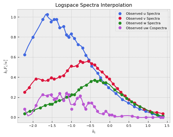
Filtering provided spectra interpolation.
==================================================

CalibrationProblem construction

We’ll use a simple neural network consisting of two layers with \(10\) neurons each, connected by a ReLU activation function. The parameters determining the network architecture can conveniently be set through the NNParameters dataclass.

Using the ProblemParameters dataclass, we indicate the eddy lifetime function \(\tau\) substitution, that we do not intend to learn the exponent \(\nu\), and that we would like to train for 10 epochs, or until the tolerance tol loss (0.001 by default), whichever is reached first.

Having set our physical parameters above, we need only pass these to the PhysicalParameters dataclass just as is done below.

Lastly, using the LossParameters dataclass, we introduce a second-order derivative penalty term with weight \(\alpha_2 = 1\) and a network parameter regularization term with weight \(\beta=10^{-5}\) to our MSE loss function.

The \(\nu\) parameter is not learned in this example and is instead fixed at \(\nu = - 1/3\).

pb = CalibrationProblem(
    nn_params=NNParameters(
        nlayers=2,
        hidden_layer_sizes=[10, 10],
        activations=[nn.ReLU(), nn.ReLU()],
    ),
    prob_params=ProblemParameters(nepochs=5),
    loss_params=LossParameters(alpha_pen2=1.0, beta_reg=1e-5),
    phys_params=PhysicalParameters(
        L=L, Gamma=Gamma, sigma=sigma, Uref=Uref, domain=domain
    ),
    logging_directory="runs/interpolating_and_fitting",
    device=device,
)
Data = datagen.Data

Calibration

Now, we fit our model. CalibrationProblem.calibrate takes the tuple Data which we just constructed and performs a typical training loop.

pb.eval(k1_data_pts)
optimal_parameters = pb.calibrate(data=Data)

pb.print_calibrated_params()

========================================
Initial loss: 7.898414848579749
========================================

100%|██████████████████████████████████████████████████████████████████| 5/5 [00:22<00:00,  4.50s/it]

========================================
Spectra fitting concluded with final loss: 0.07682391226215884
========================================
Optimal calibrated L        :  15.0558 
Optimal calibrated Γ        :   2.4787 
Optimal calibrated αϵ^{2/3} :   0.8407 
========================================

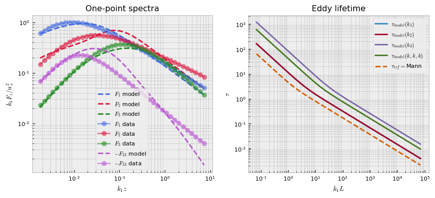
Plotting

DRDMannTurb offers built-in plotting utilities and Tensorboard integration which make visualizing results and various aspects of training performance very simple.

The following will plot our fit. As can be seen, the spectra is much smoother than the original spectra, which we investigated in the previous example.

pb.plot()

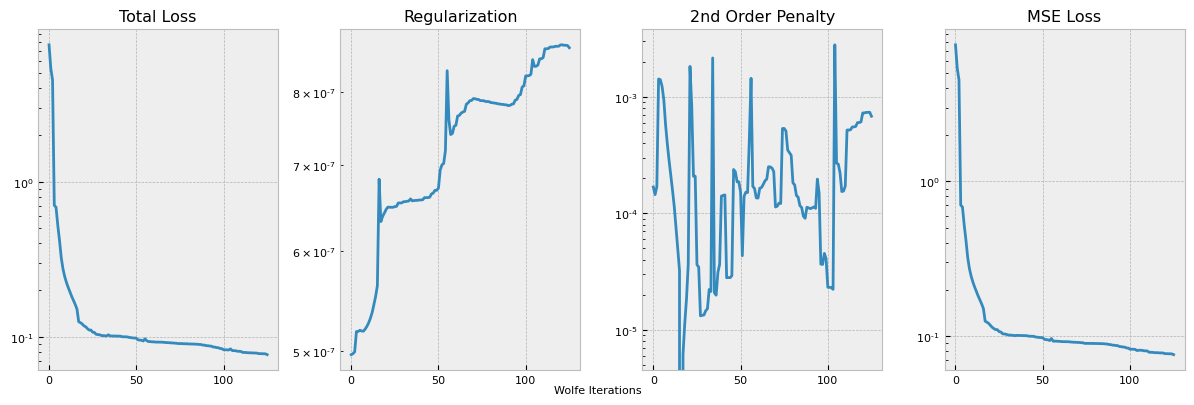
This plots out the loss function terms as specified, each multiplied by the respective coefficient hyperparameter. The training logs can be accessed from the logging directory with Tensorboard utilities, but we also provide a simple internal utility for a single training log plot.

pb.plot_losses(run_number=0)