Example 5: Custom Data Fit

In this example, we use drdmannturb to fit a simple neural network model to real-world data without any preprocessing. This involves data that are observed in the real world, specifically near a North Sea wind turbine farm. The physical parameters are determined from those measurements. Additionally, the \(\nu\) parameter is also learned. is learned for the rational function for \(\tau\) given by

\begin{align}\tau(\boldsymbol{k})=\frac{T|\boldsymbol{a}|^{\nu-\frac{2}{3}}}{\left(1+|\boldsymbol{a}|^2\right)^{\nu / 2}}, \quad \boldsymbol{a}=\boldsymbol{a}(\boldsymbol{k}).\end{align}

Import packages

First, we import the packages needed for this example, obtain the current working directory and dataset path, and choose to use CUDA if it is available.

from pathlib import Path

import numpy as np
import torch
import torch.nn as nn

from drdmannturb.enums import DataType
from drdmannturb.parameters import (
    LossParameters,
    NNParameters,
    PhysicalParameters,
    ProblemParameters,
)
from drdmannturb.spectra_fitting import CalibrationProblem, OnePointSpectraDataGenerator

path = Path().resolve()

device = "cuda" if torch.cuda.is_available() else "cpu"

if torch.cuda.is_available():
    torch.set_default_tensor_type("torch.cuda.FloatTensor")


spectra_file = (
    path / "./inputs/Spectra.dat"
    if path.name == "examples"
    else path / "../data/Spectra.dat"
)

Setting Physical Parameters

Here, we define our characteristic scales \(L, \Gamma, \alpha\epsilon^{2/3}\), the log-scale domain, and the reference height zref and velocity Uref.

domain = torch.logspace(-1, 3, 40)

L = 70  # length scale
Gamma = 3.7  # time scale
sigma = 0.04  # magnitude (σ = αϵ^{2/3})

Uref = 21  # reference velocity
zref = 1  # reference height

CalibrationProblem construction

We’ll use a simple neural network consisting of two layers with \(10\) neurons each, connected by a ReLU activation function. The parameters determining the network architecture can conveniently be set through the NNParameters dataclass.

Using the ProblemParameters dataclass, we indicate the eddy lifetime function \(\tau\) substitution, that we do not intend to learn the exponent \(\nu\), and that we would like to train for 10 epochs, or until the tolerance tol loss (0.001 by default), whichever is reached first.

Having set our physical parameters above, we need only pass these to the PhysicalParameters dataclass just as is done below.

Lastly, using the LossParameters dataclass, we introduce a second-order derivative penalty term with weight \(\alpha_2 = 1\) and a network parameter regularization term with weight \(\beta=10^{-5}\) to our MSE loss function.

Note that \(\nu\) is learned here.

pb = CalibrationProblem(
    nn_params=NNParameters(
        nlayers=2, hidden_layer_sizes=[10, 10], activations=[nn.ReLU(), nn.ReLU()]
    ),
    prob_params=ProblemParameters(
        data_type=DataType.CUSTOM, tol=1e-9, nepochs=5, learn_nu=True
    ),
    loss_params=LossParameters(alpha_pen2=1.0, beta_reg=1e-5),
    phys_params=PhysicalParameters(
        L=L,
        Gamma=Gamma,
        sigma=sigma,
        domain=domain,
        Uref=Uref,
        zref=zref,
    ),
    logging_directory="runs/custom_data",
    device=device,
)

Data from File

The data are provided in a CSV format with the first column determining the frequency domain, which must be non-dimensionalized by the reference velocity. The different spectra are provided in the order uu, vv, ww, uw where the last is the u-w cospectra (the convention for 3D velocity vector components being u, v, w for x, y, z). The k1_data_points key word argument is needed here to define the domain over which the spectra are defined.

CustomData = torch.tensor(np.genfromtxt(spectra_file, skip_header=1, delimiter=","))
f = CustomData[:, 0]
k1_data_pts = 2 * torch.pi * f / Uref
Data = OnePointSpectraDataGenerator(
    zref=zref,
    data_points=k1_data_pts,
    data_type=DataType.CUSTOM,
    spectra_file=spectra_file,
    k1_data_points=k1_data_pts.data.cpu().numpy(),
).Data

Calibration

Now, we fit our model. CalibrationProblem.calibrate takes the tuple Data which we just constructed and performs a typical training loop. The resulting fit for \(\nu\) is close to \(\nu \approx - 1/3\), which can be improved with further training.

optimal_parameters = pb.calibrate(data=Data)

pb.print_calibrated_params()

========================================
Initial loss: 5.207080587868062
========================================

100%|██████████████████████████████████████████████████████████████████| 5/5 [00:28<00:00,  5.69s/it]

========================================
Spectra fitting concluded with final loss: 0.15243641655911083
Learned nu value: 0.3917637525810459
========================================
Optimal calibrated L        :  87.5769 
Optimal calibrated Γ        :  13.3321 
Optimal calibrated αϵ^{2/3} :   0.0040 
========================================

Plotting

DRDMannTurb offers built-in plotting utilities and Tensorboard integration which make visualizing results and various aspects of training performance very simple.

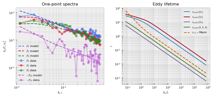
The following will plot our fit. As can be seen, the spectra is fairly noisy, which suggests that a better fit may be obtained from pre-processing the data, which we will explore in the next example.

pb.plot()

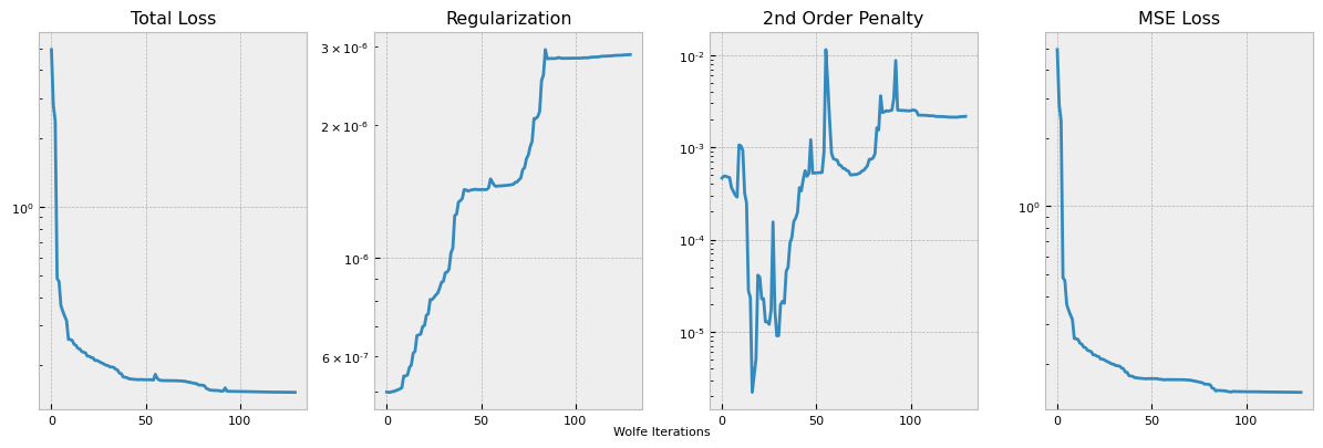
This plots out the loss function terms as specified, each multiplied by the respective coefficient hyperparameter. The training logs can be accessed from the logging directory with Tensorboard utilities, but we also provide a simple internal utility for a single training log plot.

pb.plot_losses(run_number=0)