Example 3: Adding Regularization and Penalty Terms to Fitting

This example is nearly identical to Example 2, however we use a more sophisticated loss function, introducing an additional first-order penalty term. The previous synthetic fit relied only on MSE loss and a second-order penalty.

Import packages

First, we import the packages we need for this example. Additionally, we choose to use CUDA if it is available.

import torch
import torch.nn as nn

from drdmannturb.parameters import (
    LossParameters,
    NNParameters,
    PhysicalParameters,
    ProblemParameters,
)
from drdmannturb.spectra_fitting import CalibrationProblem, OnePointSpectraDataGenerator

device = "cuda" if torch.cuda.is_available() else "cpu"

if torch.cuda.is_available():
    torch.set_default_tensor_type("torch.cuda.FloatTensor")

zref = 40  # reference height
ustar = 1.773  # friction velocity

# Scales associated with Kaimal spectrum
L = 0.59 * zref  # length scale
Gamma = 3.9  # time scale
sigma = 3.2 * ustar**2.0 / zref ** (2.0 / 3.0)  # magnitude (σ = αϵ^{2/3})

print(f"Physical Parameters: {L,Gamma,sigma}")

k1 = torch.logspace(-1, 2, 20) / zref

Physical Parameters: (23.599999999999998, 3.9, 0.8600574364289042)

Now, we construct our CalibrationProblem.

Compared to Example 2, we are instead using GELU activations and will train for fewer epochs. The more interesting difference is that we will have activated a first order term in the loss function by passing alpha_pen1 a value in the LossParameters constructor.

pb = CalibrationProblem(
    nn_params=NNParameters(
        nlayers=2,
        hidden_layer_sizes=[10, 10],
        activations=[nn.GELU(), nn.GELU()],
    ),
    prob_params=ProblemParameters(nepochs=5),
    loss_params=LossParameters(alpha_pen2=1.0, alpha_pen1=1.0e-5, beta_reg=2e-4),
    phys_params=PhysicalParameters(
        L=L, Gamma=Gamma, sigma=sigma, ustar=ustar, domain=k1
    ),
    logging_directory="runs/synthetic_3term",
    device=device,
)

In the following cell, we construct our \(k_1\) data points grid and generate the values. Data will be a tuple (<data points>, <data values>).

Data = OnePointSpectraDataGenerator(data_points=k1, zref=zref, ustar=ustar).Data

Calibration

Now, we fit our model. CalibrationProblem.calibrate takes the tuple Data which we just constructed and performs a typical training loop.

optimal_parameters = pb.calibrate(data=Data)

pb.print_calibrated_params()

========================================
Initial loss: 0.04272825028614858
========================================

100%|██████████████████████████████████████████████████████████████████| 5/5 [00:13<00:00,  2.66s/it]

========================================
Spectra fitting concluded with final loss: 0.0055182869502642526
========================================
Optimal calibrated L        :  25.9472 
Optimal calibrated Γ        :   4.5198 
Optimal calibrated αϵ^{2/3} :   0.8015 
========================================

Plotting

DRDMannTurb offers built-in plotting utilities and Tensorboard integration which make visualizing results and various aspects of training performance very simple. The training logs can be accessed from the logging directory with Tensorboard utilities, but we also provide a simple internal utility for a single training log plot.

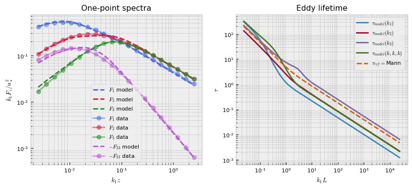
The following will plot our fit.

pb.plot()

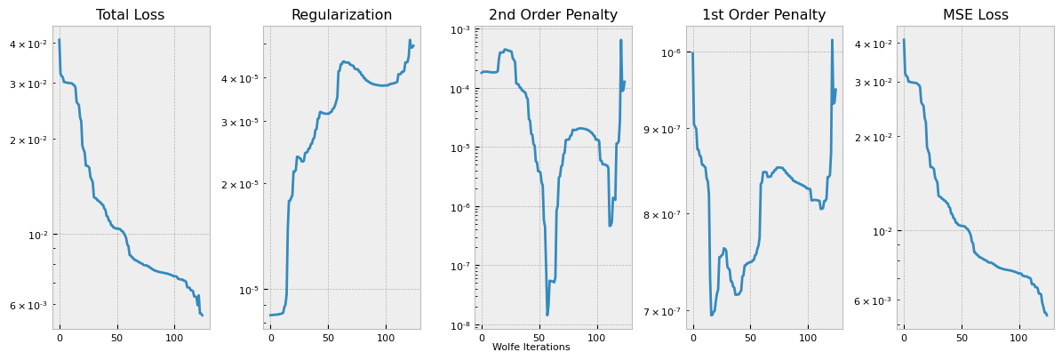
This plots out the loss function terms as specified, each multiplied by the respective coefficient hyperparameter.

pb.plot_losses(run_number=0)