Example 4: Changing MLP Architecture and Fitting

This example is nearly identical to the Synthetic Data fit, however we use a different neural network architecture in hopes of obtaining a better spectra fitting. The same set-up for fitting the Kaimal spectra is used here as in Examples 2 and 3. The only difference here is in the neural network architecture. Although certain combinations of activation functions, such as GELU result in considerably improved spectra fitting and terminal loss values, the resulting eddy lifetime functions may be non-physical.

Import packages

First, we import the packages we need for this example. Additionally, we choose to use CUDA if it is available.

import torch
import torch.nn as nn

from drdmannturb.parameters import (
    LossParameters,
    NNParameters,
    PhysicalParameters,
    ProblemParameters,
)
from drdmannturb.spectra_fitting import CalibrationProblem, OnePointSpectraDataGenerator

device = "cuda" if torch.cuda.is_available() else "cpu"

if torch.cuda.is_available():
    torch.set_default_tensor_type("torch.cuda.FloatTensor")

Set up physical parameters and domain associated with the Kaimal spectrum. We perform the spectra fitting over the \(k_1\) space \([10^{{-1}}, 10^2]\) with 20 points.

zref = 40  # reference height
ustar = 1.773  # friction velocity

# Scales associated with Kaimal spectrum
L = 0.59 * zref  # length scale
Gamma = 3.9  # time scale
sigma = 3.2 * ustar**2.0 / zref ** (2.0 / 3.0)  # magnitude (σ = αϵ^{2/3})

print(f"Physical Parameters: {L,Gamma,sigma}")

k1 = torch.logspace(-1, 2, 20) / zref

Physical Parameters: (23.599999999999998, 3.9, 0.8600574364289042)

Now, we construct our CalibrationProblem.

Compared to Examples 2 and 3, we are using a more complicated neural network architecture. This time, specifically, our network will have 4 layers of width 10, 20, 20, 10 respectively, and we use both GELU and RELU activations. We have prescribed more Wolfe iterations. Finally, this task is considerably more difficult than before since the exponent of the eddy lifetime function \(\nu\) is to be learned. Much more training may be necessary to obtain a close fit to the eddy lifetime function. Interestingly, learning this parameter results in models that more accurately describe the spectra of Mann turbulence than using the Mann model itself.

pb = CalibrationProblem(
    nn_params=NNParameters(
        nlayers=4,
        # Specifying the activations is done as in Examples 2 and 3.
        hidden_layer_sizes=[10, 20, 20, 10],
        activations=[nn.ReLU(), nn.GELU(), nn.GELU(), nn.ReLU()],
    ),
    prob_params=ProblemParameters(nepochs=25, wolfe_iter_count=20),
    loss_params=LossParameters(alpha_pen2=1.0, beta_reg=1.0e-5),
    phys_params=PhysicalParameters(
        L=L, Gamma=Gamma, sigma=sigma, ustar=ustar, domain=k1
    ),
    logging_directory="runs/synthetic_fit_deep_arch",
    device=device,
)

Data Generation

In the following cell, we construct our \(k_1\) data points grid and generate the values. Data will be a tuple (<data points>, <data values>).

Data = OnePointSpectraDataGenerator(data_points=k1, zref=zref, ustar=ustar).Data

Training

Now, we fit our model. CalibrationProblem.calibrate() takes the tuple Data which we just constructed and performs a typical training loop.

optimal_parameters = pb.calibrate(data=Data)

pb.print_calibrated_params()

========================================
Initial loss: 0.04528620934615529
========================================

100%|████████████████████████████████████████████████████████████████| 25/25 [01:44<00:00,  4.16s/it]

========================================
Spectra fitting concluded with final loss: 0.0028603860525603627
========================================
Optimal calibrated L        :  23.1940 
Optimal calibrated Γ        :   4.5563 
Optimal calibrated αϵ^{2/3} :   0.8238 
========================================

Plotting

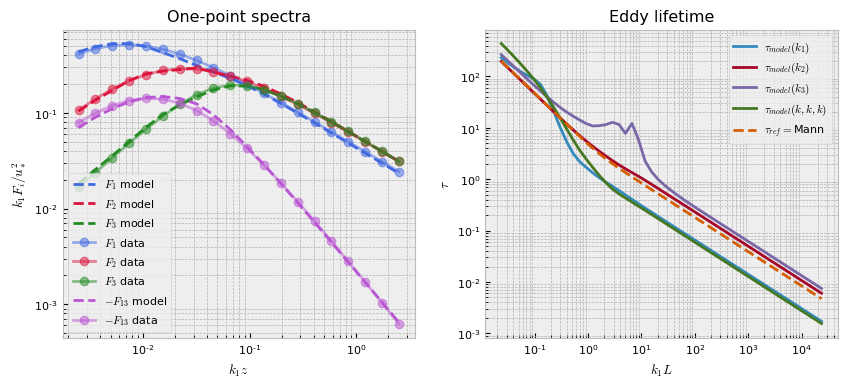
Lastly, we’ll use built-in plotting utilities to see the fit result.

pb.plot()

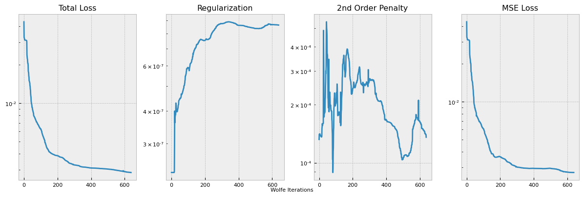
This plots the loss function terms as specified, each multiplied by the respective coefficient hyperparameter. The training logs can be accessed from the logging directory with Tensorboard utilities, but we also provide a simple internal utility for a single training log plot.

pb.plot_losses(run_number=0)